Use Cases
This page demonstrates several use cases of Simantha that extend the behavior of the basic manufacturing objects.
Condition-Monitored Machine
In this example we demonstrate the extensibility of the simantha.Machine class. We implement a condition-monitored machine whose health state is not precisely known, but is observed with the addition of some random noise. The ConditionMonitoredMachine extends simantha.Machine and includes a method for observing the health signal. We must also implement a new simulation event by extending the simantha.simulation.Event class.
import random

import numpy as np

from simantha import Source, Machine, Sink, Maintainer, System, simulation, utils
We assign a priority of 5.5 to the sensing event so that it is executed in the proper order. In this cases, we observe the signal just after a potential degradation event on the machine.
class SensingEvent(simulation.Event):
    def get_action_priority(self):
        return 5.5
We add a Gaussian noise term to the true health state of the machine to obtain the observed health signal. We observe the health signal at regular intervals as specified by the sensing_interval parameter. We also store these observations in the sensor_data attribute of the machine.
We schedule the first sensing event using the initialize_addon_process method which is called at the beginning of a simulation run. Once the event is executed by calling the sense method, we schedule the next sensing event. If the machine undergoes maintenance, we must restart the sensing process using the repair_addon_process method.
class ConditionMonitoredMachine(Machine):
    def __init__(self, sensing_interval=1, sensor_noise=0, **kwargs):
        self.sensing_interval = sensing_interval
        self.sensor_noise = sensor_noise
        self.sensor_data = {'time': [], 'reading': []}

        super().__init__(**kwargs)

    def initialize_addon_process(self):
        self.env.schedule_event(
            time=self.env.now,
            location=self,
            action=self.sense,
            source=f'{self.name} initial addon process',
            event_type=SensingEvent
        )

    def repair_addon_process(self):
        self.env.schedule_event(
            time=self.env.now,
            location=self,
            action=self.sense,
            source=f'{self.name} repair addon process at {self.env.now}',
            event_type=SensingEvent
        )

    def sense(self):
        self.sensor_reading = self.health + np.random.normal(0, self.sensor_noise)

        self.sensor_data['time'].append(self.env.now)
        self.sensor_data['reading'].append(self.sensor_reading)

        self.env.schedule_event(
            time=self.env.now+self.sensing_interval,
            location=self,
            action=self.sense,
            source=f'{self.name} sensing at {self.env.now}',
            event_type=SensingEvent
        )
We can now instantiate a ConditionMonitoredMachine and create a system to simulate.
degradation_matrix = utils.generate_degradation_matrix(h_max=10, p=0.1)
cm_distribution = {'geometric': 0.1}

source = Source()
M1 = ConditionMonitoredMachine(
    name='M1',
    cycle_time=2,
    degradation_matrix=degradation_matrix,
    cm_distribution=cm_distribution,
    sensing_interval=2,
    sensor_noise=1
)
sink = Sink()

source.define_routing(downstream=[M1])
M1.define_routing(upstream=[source], downstream=[sink])
sink.define_routing(upstream=[M1])

system = System(objects=[source, M1, sink])

random.seed(1)
system.simulate(simulation_time=6*60)

# Output
# Simulation finished in 0.03s
# Parts produced: 167
We can print the first few rows of M1.sensor_data to see how the observations compare to the underlying true health value.
rows = 12
print('\ntime  health  sensor reading')
for time, reading in zip(
    M1.sensor_data['time'][:rows], M1.sensor_data['reading'][:rows]
):
    timestamp = max([t for t in M1.health_data['time'] if t <= time])
    idx = M1.health_data['time'].index(timestamp)
    health = M1.health_data['health'][idx]
    print(f'{time:<4}  {health:<3}    {reading:>8.4f}')
Which gives the output:
Simulation finished in 0.03s
Parts produced: 167

time  health  sensor reading
0     0       -1.2002
2     0        1.6348
4     0        1.2738
6     0        1.2323
8     0       -1.5130
10    0       -0.6196
12    0        0.4308
14    0        0.6227
16    0       -0.1939
18    1        1.4526
20    2        3.3068
22    2       -0.0844
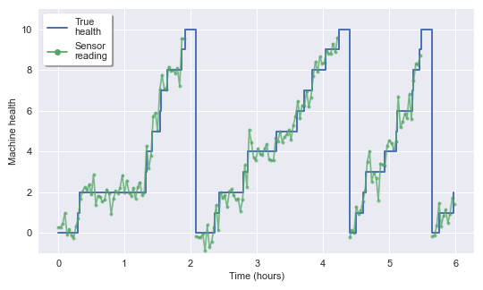
The figure below shows the true health of a single machine compared to the observed sensor readings over a period of six hours.
Alternate Maintenance Policy
In this example we implement a Maintainer that uses a longest processing time first (LPT) rule for scheduling maintenance instead of the default first-in, first-out rule. If we consider two types of maintenance jobs, preventive and corrective, then an LPT rule prioritizes corrective jobs since their duration is greater on average.
First, we create a LptMaintainer class that inherits simantha.Maintainer and overrides the choose_maintenance_action method.
import random

from simantha import Source, Machine, Buffer, Sink, Maintainer, System, utils

def expected_repair_time(machine):
    # Returns the expected duration of the pending repair
    if machine.failed:
        # Machine is awaiting corrective maintenance
        return machine.cm_distribution.mean
    else:
        # Machine is awaiting preventive maitenance
        return machine.pm_distribution.mean

class LptMaintainer(Maintainer):
    """Chooses the maintenance action with the longest expected duration first."""
    def choose_maintenance_action(self, queue):
        return max(queue, key=expected_repair_time)
Then we construct a simple serial line with three machines subject to a Markov degradation process.
degradation_matrix = [
    [0.9, 0.1, 0.,  0.,  0. ],
    [0.,  0.9, 0.1, 0.,  0. ],
    [0.,  0.,  0.9, 0.1, 0. ],
    [0.,  0.,  0.,  0.9, 0.1],
    [0.,  0.,  0.,  0.,  1. ]
]

source = Source()
M1 = Machine(
    name='M1',
    cycle_time=1,
    degradation_matrix=degradation_matrix,
    cm_distribution={'geometric': 0.1}
)
B1 = Buffer(capacity=10)
M2 = Machine(
    name='M2',
    cycle_time=1,
    degradation_matrix=degradation_matrix,
    cm_distribution={'geometric': 0.075}
)
B2 = Buffer(capacity=10)
M3 = Machine(
    name='M3',
    cycle_time=1,
    degradation_matrix=degradation_matrix,
    cm_distribution={'geometric': 0.05}
)
sink = Sink()

source.define_routing(downstream=[M1])
M1.define_routing(upstream=[source], downstream=[B1])
B1.define_routing(upstream=[M1], downstream=[M2])
M2.define_routing(upstream=[B1], downstream=[B2])
B2.define_routing(upstream=[M2], downstream=[M3])
M3.define_routing(upstream=[B2], downstream=[sink])
sink.define_routing(upstream=[M3])

objects = [source, M1, B1, M2, B2, M3, sink]
maintainer = LptMaintainer(capacity=1)

system = System(objects, maintainer)
Finally, we simulate the system for one week.
random.seed(1)
system.simulate(simulation_time=utils.WEEK)

# Output:
# Simulation finished in 0.74s
# Parts produced: 4566